Abstract: The sensor signal of a magnetic Thickness Gauge is a strongly nonlinear function, and its accurate fitting is the basis for high-precision measurement of the Thickness Gauge. It is simulated by BP network
Combination is a new attempt. In this paper, the BP network based on Bayesian regularization LM algorithm is applied to the research of Thickness Gauge, and the neuron training program is compiled. The trained neurons are used in the software design of the Thickness Gauge. The simulation experiment and the actual test results of the Thickness Gauge show that, compared with the square polynomial and piecewise linear fitting algorithms, the algorithm can improve the accuracy and has good general performance. It can achieve practical accuracy with less training steps.
Keywords: coating, thickness measurement, neural network, curve fitting
Coating non-destructive testing has been commercialized, but as far as the coating thickness testing equipment designed based on the principle of electromagnetic induction, there are still the following shortcomings [1]: The instrument has a large system error; the change of the measurement environment (such as temperature, medium, electric field, etc.) will cause the instrument to have a large measurement error; the influence of different ferromagnetic substrates or working shapes on the measurement is not easy to eliminate; it is difficult to apply The coating thickness is dynamically monitored during the process. Due to the non-linearity of the measurement principle, small disturbances will affect the measurement accuracy and greatly affect the performance indicators of the instrument. In the Thickness Gauge, in order to reduce the measurement error (change of temperature and medium), it is often necessary to calibrate the instrument and re-fit the sensor signal curve. The existing fitting methods have their limitations and are not very good meet high performance requirements. The BP network and its variants are the core of the forward network, and embody the most essential part of the artificial neural network. BP neural network can approximate any continuous function or mapping relationship with any given precision. Using the strong nonlinear mapping ability of the artificial neural network to fit the relationship curve between the induced voltage e of the Thickness Gauge sensor and the coating thickness d, a high fitting accuracy can be obtained. In this paper, the improved LM algorithm based on the Bayesian regularization method is used for curve fitting, and a good fitting performance and high network generalization ability are obtained.
working principle
The electromagnetic induction method to detect the surface coating thickness of ferromagnetic substrate and non-ferromagnetic material is a non-destructive testing method for surface coating thickness designed according to the obvious difference in magnetic permeability of the substrate and coating based on the essential difference in magnetic properties. Since the magnetic resistance of the substrate is much smaller than that of the coating, if the thickness of the coating is different, the distance between the probe and the surface of the substrate is different, so the magnetic flux generated by the exciting coil of the probe is different, resulting in the induced voltage in the measuring coil on the probe different. Coating thickness information can be obtained by measuring the difference in this induced voltage signal. Under satisfactory conditions, the induced voltage e has a definite analytical relationship with the coating thickness d.
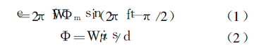
In the formula, e-induced voltage (unit V), f-magnetic field change frequency (unit rad/s), W-measurement coil turns, Υm-maximum magnetic flux (unit Wb), i-coil current (unit A), μ - magnetic permeability (unit H/m), S - coil area (unit m2), d - coating thickness (unit m).
The function d=f(e) is a strongly nonlinear function, and there are many ways to fit it[4][5], such as modified arctangent function fitting, high degree polynomial fitting, hyperbolic function, cubic spline Function piecewise interpolation, linear multi-section interpolation. The main problem of using curve fitting is that the measurement accuracy is difficult to guarantee. There are too many constraints in polynomial interpolation, and there is no theoretical basis for determining the number of times. If the number is too high, "Runge phenomenon" will appear; cubic spline function segments have "unreasonable fluctuations"; linear multi-segmentation also has problems that cannot be overcome. Problem, in order to obtain linear sensing signal [1], the sensor adopts high-frequency resonance technology, and the operating frequency of the sensor is in the range of 30-80kHz. Excessively high operating frequency of the sensor leads to poor adaptability to the substrate. When the material of the substrate is different (such as low-carbon steel, high-carbon steel, etc., that is, the magnetic permeability of the material is different) it will have a greater impact on the measurement results. The shape (such as the size of the radius of curvature, etc.) has poor adaptability and is not suitable for measuring the thickness of non-metallic coatings.
LM Algorithm Based on Bayesian Regularization
The main idea of the BP algorithm is to divide the learning process into two stages: the forward propagation process, the given input information is processed layer by layer through the input layer through the hidden layer and the actual output of each unit is calculated; the error back propagation process, if If the expected output value is not obtained at the output layer, the error between the actual output and the expected output is recursively calculated layer by layer, and the weight is adjusted according to the error. The LM algorithm [6] [7] is an improved BP algorithm, which has a second-order training speed, but does not need to directly calculate the Hessian matrix. For the LM learning algorithm, if the objective function of the processing problem is in the form of the sum of squares, the Hessian matrix and the gradient function can be approximated by the formula H=JTJ and g=JTe, where J is the Jacobian matrix, which is the network weight and the network The first derivative of the bias, e is the network vector error. During the entire iterative calculation process, the LM algorithm is expressed by the following approximate value of the Hessian matrix:
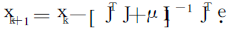
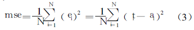
If μ is zero, the above formula is the Newton method that approximates the Hessian matrix. If the value of μ is large, it becomes the fastest gradient descent method with a small step size. When the approximation error is minimized, the quasi-Newton method is faster and more accurate, and the performance is as close as possible to the Newton method. When each iteration is successful, the value of μ will decrease, and only when each tentative iteration increases the objective function, the value of μ will increase, so that in each iteration of the algorithm, the objective function will decrease. An over-trained neural network may achieve a high matching effect on the training sample set, but it may produce an output that is quite different from the target vector for a new input sample vector, that is, the generalization ability of the neural network is poor. In this paper, a method based on Bayesian regularization is used to improve the generalization ability of the LM algorithm. The training performance function of the neural network often adopts the mean square error mse, namely:
In the regularization method, the network performance function is improved into the following form:
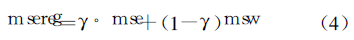
In the formula, γ is the proportional coefficient, and msw is the average value of the sum of squares of all network weights, namely
By adopting the new performance index function, the network can have smaller weights while ensuring the network training error is as small as possible, that is, the effective weights of the network are as few as possible, which is equivalent to automatically reducing the size of the network. Conventional regularization methods are usually difficult to determine the size of the proportional coefficient λ, while the Bayesian regularization method can adaptively adjust the size of γ during network training and make it better, so that the trained network has Better ability to promote.
BP Algorithm for Curve Fitting of Thickness Gauge Sensor
1. Existing fitting algorithm
In the design of Thickness Gauges, two fitting functions are commonly used, namely the square coefficient polynomial and the multi-segment straight line method:
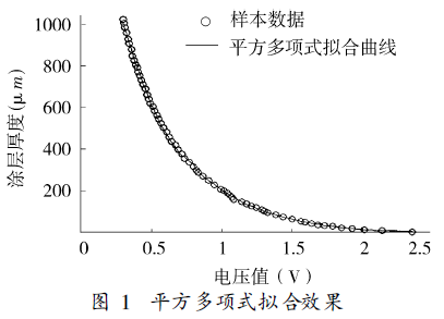
Using multi-segment straight line fitting requires a linear sensor signal, which is generally difficult to meet. The square polynomial is fitted by the least square method, which overcomes the shortcomings of the numerical oscillation of the high-order polynomial, ensures the smoothness of the curve, and has a certain fitting accuracy. Its fitting effect is shown in Figure 1.
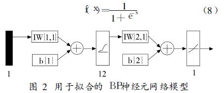
2. Bayesian regularized LM fitting algorithm The Bayesian regularized LM fitting algorithm for sensor signals of magnetic Thickness Gauges, its BP neuron network model is shown in Figure 2. It is a BP network with single input, single output and single hidden layer, the number of hidden layer nodes is set to 12, and the activation function is logsig. That is:
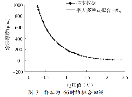
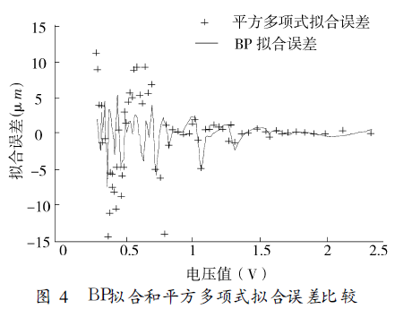
When the number of samples is 66 and the training step size is selected as 50, the fitting effect is shown in Figure 3. The comparison between BP fitting and square polynomial fitting error is shown in Fig. 4. The Bayesian regularized LM fitting algorithm has higher fitting accuracy, which can fully satisfy the measurement error of ±(1%H+0.7)μm(H is the accuracy requirement of the measured coating thickness). Will
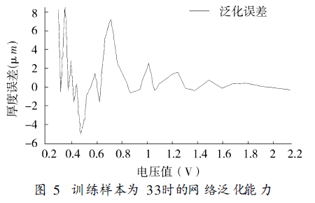
The samples are divided into two groups, 33 samples are used to train the network, and the other 33 samples are used to test the generalization ability of the algorithm, and good results have been achieved. Its generalized error curve is shown in Fig. 5.
in conclusion
The BP network based on the Bayesian regularized LM algorithm is applied to the fitting of the sensor signal of the Thickness Gauge. The practical results show that compared with the quadratic polynomial and piecewise linear fitting algorithms, the algorithm improves the fitting accuracy and has good Under the condition of satisfying the practical accuracy of the instrument, the number of training steps is less and the smoothness is better.